Shot quality on an NBA court

Where does a team take its shots, and does it make more of them than an average team would from the same spots? This recipe answers both for every field goal attempt of the 2025-26 NBA regular season, with three SportsDataverse packages working together:

• sportsdataverse-py loads the shots (the stats-API shot file the SportsDataverse publishes on GitHub, so nothing calls stats.nba.com),
• sdvplot moves them onto sportypy's court and supplies team colors and logos,
• sportypy draws the court and bins the shots onto it with hexbin.

To run it yourself: pip install sportypy sportsdataverse "sdvplot[surfaces]", or from a clone of the repository, uv run --group cookbook jupyter lab.

Open in Colab · View the notebook on GitHub

import matplotlib.pyplot as plt
import polars as pl
import sportsdataverse.nba as nba
from matplotlib.colors import TwoSlopeNorm

import sdvplot
from sportypy.surfaces.basketball import NBACourt

# print tables as markdown, so the docs site shows them as tables
pl.Config.set_tbl_formatting("ASCII_MARKDOWN")
pl.Config.set_tbl_hide_column_data_types(True)
pl.Config.set_tbl_hide_dataframe_shape(True)
SEASON = 2025  # this loader names a season by the year it starts: 2025 is 2025-26

1. Every shot, on sportypy's frame

The stats API reports a shot's location in tenths of a foot with the hoop at the origin. sportypy's court is in feet with the origin at center court. sdvplot.court_coords converts one to the other and adds court_x and court_y; every shot lands on the left half of the court. A shot's value is points when it goes in and 0 when it does not.

shots = sdvplot.court_coords(
    nba.load_nba_stats_shots(seasons=SEASON).filter(pl.col("season_type_id") == "2")  # 2: regular season
).with_columns(
    made=pl.col("shot_result") == "Made",
    points=pl.when(pl.col("shot_result") == "Made").then(pl.col("shot_value")).otherwise(0),
)
print(f"{shots.height:,} shots by {shots['team_tricode'].n_unique()} teams")
print(shots.select("team_tricode", "player_name", "shot_value", "shot_distance", "court_x", "court_y", "points").head(3))

219,159 shots by 30 teams

team_tricode	player_name	shot_value	shot_distance	court_x	court_y	points
HOU	Sengun	3	25	-23.85	-17.9	0
OKC	Holmgren	2	1	-40.45	0.0	2
HOU	Thompson	3	23	-41.75	23.3	0

2. Where the league shoots

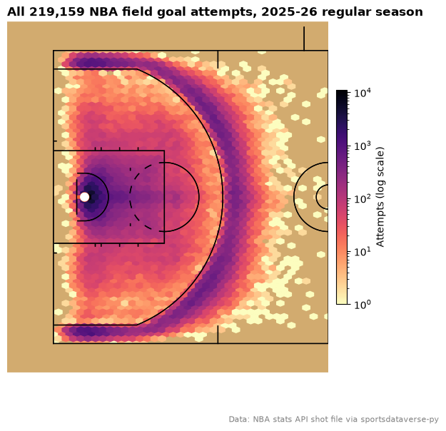
NBACourt.hexbin bins the points into hexagons sized in feet (binsize) and clips them to the court. display_range="defense" draws only the left half, where every shot is. The log color scale keeps the rim, which has many times more attempts than anywhere else, from washing out the rest: the rim, the corners and the arc are the darkest, and the long two in between takes about a tenth as many shots as the arc.

court = NBACourt()
fig, ax = plt.subplots(figsize=(7, 6.5))
court.draw(ax=ax, display_range="defense")
hexes = court.hexbin(shots["court_x"], shots["court_y"], binsize=1.5, bins="log", cmap="magma_r", mincnt=1, ax=ax)
fig.colorbar(hexes, ax=ax, shrink=0.6, pad=0.02, label="Attempts (log scale)")
ax.set_title(f"All {shots.height:,} NBA field goal attempts, 2025-26 regular season", loc="left", fontweight="bold")
fig.text(0.99, 0.01, "Data: NBA stats API shot file via sportsdataverse-py", ha="right", fontsize=8, color="grey")
plt.show()

3. What a shot is worth from each distance

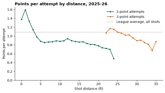
The league's average points per attempt at each distance (in whole feet, with everything past 35 feet pooled) and shot value is the baseline for the rest of the recipe: an average team's expected return on the same shot. A two at the rim is worth well over a point; the long two is the worst shot on the floor, and a step back behind the arc is worth more than a step in.

expected = (
    shots.with_columns(dist=pl.col("shot_distance").clip(upper_bound=35))
    .group_by("dist", "shot_value")
    .agg(attempts=pl.len(), xpts=pl.col("points").mean())
    .filter(pl.col("attempts") >= 50)
    .sort("dist")
)

fig, ax = plt.subplots(figsize=(8, 4))
for value, color in ((2, "#006838"), (3, "#e06000")):
    line = expected.filter(pl.col("shot_value") == value)
    ax.plot(line["dist"], line["xpts"], marker="o", ms=3, color=color, label=f"{value}-point attempts")
ax.axhline(shots["points"].mean(), color="grey", lw=0.8, ls="--", label="League average, all shots")
ax.set(xlabel="Shot distance (ft)", ylabel="Points per attempt", ylim=(0, None))
ax.spines[["top", "right"]].set_visible(False)
ax.legend(frameon=False)
ax.set_title("Points per attempt by distance, 2025-26", loc="left", fontweight="bold")
plt.show()

4. Points over expected, shot by shot

Join the baseline back onto every shot and each one gets an expected value, xpts. A make from a spot where the league scores 1.1 points per attempt is worth 2 - 1.1 = +0.9 over expected, a miss there -1.1. Summed over a season, that separates teams that take good shots (a high xpts per attempt) from teams that make the shots they take (a high over per attempt).

shots = shots.with_columns(dist=pl.col("shot_distance").clip(upper_bound=35)).join(
    expected.select("dist", "shot_value", "xpts"), on=["dist", "shot_value"], how="left"
).with_columns(over=pl.col("points") - pl.col("xpts"))

teams = (
    shots.drop_nulls("xpts")
    .group_by("team_tricode")
    .agg(attempts=pl.len(), pts=pl.col("points").mean(), xpts=pl.col("xpts").mean(), over=pl.col("over").mean())
    .sort("over", descending=True)
)
with pl.Config(float_precision=3, tbl_rows=10):
    print(pl.concat([teams.head(5), teams.tail(5)]))

team_tricode	attempts	pts	xpts	over
LAL	6863	1.146	1.069	0.077
DEN	7196	1.154	1.079	0.075
BOS	7398	1.106	1.052	0.053
LAC	6857	1.118	1.072	0.045
MIL	7012	1.131	1.093	0.037
PHI	7404	1.061	1.098	-0.037
CHI	7417	1.095	1.146	-0.051
POR	7389	1.067	1.119	-0.051
BKN	6933	1.041	1.106	-0.065
NOP	7420	1.054	1.122	-0.068

5. Where the best and worst shooting teams beat the league

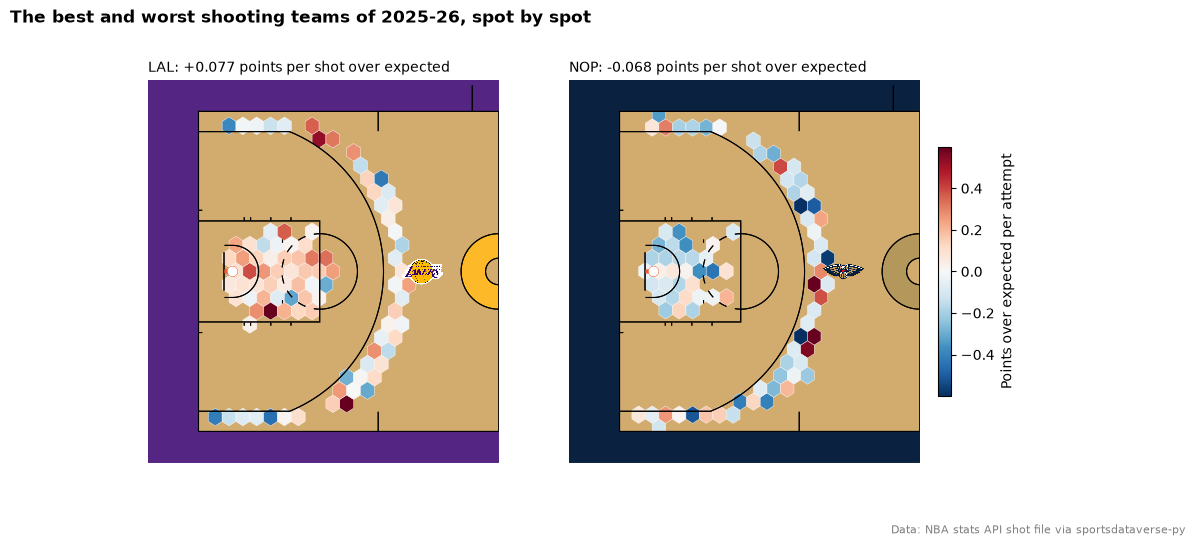
Pass over as the hexbin's values and each hexagon shows the team's average points over expected there (mincnt leaves out spots with too few attempts to say). A diverging palette centered on zero puts the league average in white. The courts are painted in each team's colors from sdvplot (team_colors), handed to sportypy as color_updates, and add_logos puts the team's logo beyond the arc.

best, worst = teams["team_tricode"][0], teams["team_tricode"][-1]
norm = TwoSlopeNorm(vcenter=0, vmin=-0.6, vmax=0.6)

fig, axes = plt.subplots(1, 2, figsize=(12, 5.4))
for ax, team in zip(axes, (best, worst)):
    primary = sdvplot.team_colors("nba", team)
    secondary = sdvplot.team_colors("nba", team, which="secondary")
    court = NBACourt(color_updates={"court_apron": primary, "center_circle_fill": secondary})
    court.draw(ax=ax, display_range="defense")
    mine = shots.filter((pl.col("team_tricode") == team) & pl.col("over").is_not_null())
    hexes = court.hexbin(mine["court_x"], mine["court_y"], values=mine["over"], binsize=4, mincnt=20,
                         cmap="RdBu_r", norm=norm, edgecolors="white", linewidths=0.3, ax=ax)
    sdvplot.add_logos(ax, [-12], [0], [team], league="nba", height=0.12, zorder=30)
    row = teams.filter(pl.col("team_tricode") == team).row(0, named=True)
    ax.set_title(f"{team}: {row['over']:+.3f} points per shot over expected", loc="left", fontsize=10)
fig.colorbar(hexes, ax=axes, shrink=0.6, pad=0.02, label="Points over expected per attempt")
fig.suptitle("The best and worst shooting teams of 2025-26, spot by spot", x=0.01, ha="left", fontweight="bold")
fig.text(0.99, 0.01, "Data: NBA stats API shot file via sportsdataverse-py", ha="right", fontsize=8, color="grey")
plt.show()

Where to go next

• The NBACourt reference lists every feature color_updates can repaint, and the plotting reference every option of hexbin, heatmap and contour.
• sdvplot's surfaces and shot charts cookbook draws single-player shot charts on team-colored courts in one call.
• Swap nba for wnba (load_wnba_stats_shots, sdvplot.court_coords and sportypy's WNBACourt) and the recipe runs unchanged on the WNBA.